
Molecular Replacement Tutorial
This tutorial solves one protein structure using the structure of a similar protein.The Problem
The example is to solve cardiotoxin which is:This protein is now in the PDB as 1tgx.pdb (solved by A.Bilwes,B.Rees,D.Moras J.Mol.Biol. 1994, V239, p-122).
Outline of the Method
1) Make an estimate of the number of molecules in the asymmetric unit so we know how many molecules to look for with the molecular replacement programs.2) Look at our experimental data - are there any problems?
3) Run molecular replacement program to find solutions.
4) Refine the phases using NCS (non-cystallographic symmetry) phased refinement.
The Data Files
Files in directory $DATAmodel.pdb -
contains coordinates of the model we will use to solve cardiotoxin.
cardiotoxin.mtz -
contains the experimental data.
Files in the directory $RESULTS
matthews.log
- the log file from Cell Content Analysis
For next steps see the picture here
1.1 Change to the Coordinate Utilities
module. Select the Cell Content Analysis
task.
1.2 Select the MTZ file - the program will read
the space group and cell dimensions from the MTZ file (so you do not need
to type them in):
MTZ file
DATA
cardiotoxin.mtz.
1.3 Enter the molecular weight of the protein. The
protein has 60 residues and we say average residue weight is 100 Dalton.
So
Molecular weight of protein 6000.
1.4 Click the Run Now button.
1.5 Look at the output in the window - it shows a table
of the Matthew's coefficient and percentage solvent content dependent on
the number of molecules that are in the asymmetric unit.
1.6) Close the Cell Content
Analysis window.
a) Create a Patterson map and search it for peaks.
We expect a big peak at the origin (position 0,0,0) but if there is another
big peak (perhaps about 0.25 the size of the origin peak) then perhaps
there is translation between the molecules in the asymmetric unit
and it will be more difficult to solve.
(The theory behind this is explained on the web site of Bernhard
Rupp:
http://www-structure.llnl.gov/xray/101index.html
For more information, go to the section on Phasing Techniques on
this website, and click on NCS with native Patterson maps)
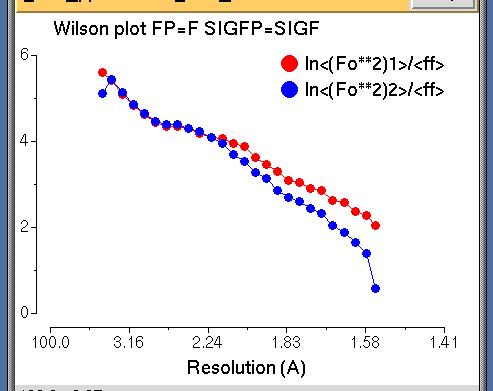
b) Create a Wilson plot which is an indication of the
self consistency of the data. Also find the average B-value of the
data - this can be used to help the molecular replacement program.
For the next steps look at picture here
2.1) Change to the Molecular Replacement
module and select the Analyse Data for MR
task.
2.2) Select the input experimental data
MTZ in
DATA cardiotoxin.mtz
2.3) Select input model:
PDB in DATA
model.pdb
2.4) Enter the Number of residues in the asymmetric
unit - this is:
number of molecules in asymmetric unit *
number of residues per molecule
= 3 * 60
= 180
Number of residues in asymmetric
unit 180
2.5) Run the
job. You can now Close the Analyse
Data window.
2.6) Look at the log file when the job has finished.
In the main CCP4i window click on the job called mr_analyse
and then from menu View Files from Job select
View Log File. In the log file is output
from the programs FFT which created the Patterson map and Peakmax
which searched for peaks in the map. To find what we want
click on the Find button and enter the text
List of peaks. You can now see table
like this:
Hints
In fact the values you get may be different, for example:
You may also see a different number of peaks, for example:
The difference is an effect of the width of the Patterson origin peak being
related to the resolution range of data included when generating the Patterson
map. At lower resolutions the origin peak may overlap neighbouring grid points
in the map, and result in apparent extra peaks in these adjacent positions.
Including higher resolution data narrows the origin peak and reduces the
effect; try changing the high resolution limit from 4.0 A to 3.0 A in the
Define Map folder, and re-run.
2.7) Now go to the bottom of the log file where
you will see:
Wilson Plot
This is a usual Wilson plot - no problems here!
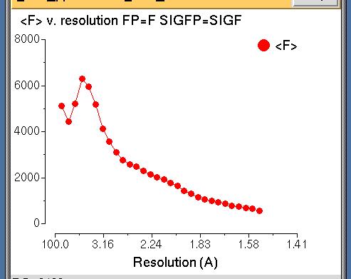
Amplitude Analysis v. Resolution
This plot is usual shape for amplitude
versus resolution plot with 'water' peak at about 4A.
Average B v. Residue
This shows the difference from the
mean - in this PDB file all the B values are set to 20.
This is not interesting for this protein.
Quit from
the two windows which display the log file and the graphs.
For the next few steps look at picture here
3.1) From the Molecular
Replacement menu select MolRep
- auto MR
3.2) The default mode for
running MolRep is good:
Do molecular
replacement performing rotation
and translation function
3.3) Select the input experimental
data file.
MTZ in DATA
cardiotoxin.mtz.
3.4) Select the input model.
Model in
DATA model.pdb
3.5) Look down the window a little:
set the
Search for
3 monomers in
the asymmetric unit.
3.6) From the Run
menu select Run
Now.
MolRep will take a long time to
run - if it is too long you can see the output files: $RESULTS/molrep.log
and $RESULTS/mr_model_molrep1.pdb.
Go to directory
RESULTS
then
File
molrep.log
and the click on Display
and Exit
The log file lists many possible
solutions. After the rotation function:
After a translation function:
The program runs the translation function three times
to find three different molecules. For the second run of the translation
function it will take the best solution from the first run and try to find
another molecule which will fit well with the first solution. For
the third run of the translation function it will keep the best solution
from the first run and the second run and try to find molecule number three.
It is not possible to say what is a good score - this
will depend on many things but it is good if the best score (the correlation
factor in the column labelled Corr) is much bigger than the second
best score. When you are looking for several molecules the best score
for the first (and perhaps second) molecule will not be very good but you
hope that the best score for all three molecules is much better than for
other possible solutions.
3.7) The output file mr_model_molrep1.pdb
contains three copies of the input model moved to the right positions in
the asymmetric unit. The three
molecules will pack together something like this.
For the next few steps look at the picture here
4.1) Go to the Refinement
module and chose Run Refmac5
4.2) Enter the name of the data file:
MTZ in
DATA
cardiotoxin.mtz
Enter the name of the input files - this is the coordinate
file output from MolRep:
PDB in
RESULTS model_molrep1.pdb
If you have not run molrep, use the model_molrep1.pdb file found in DATA:
PDB in
DATA model_molrep1.pdb 4.3) Now you must tell the program that it must
keep the non-crystallographic symmetry by keeping the three chains
similar. Click on the line with the folder title
Non-crystallographic Symmetry
4.4) Click on the button
Add non-X restraint
4.5) Click three times on the button
Add chain
4.6) Now set up like this:
Restrain together chain A
4.7) Make sure you are not creating a data harvesting file. Select:
Do not create harvest file
from the Data Harvesting section. 4.8) Run the program by clicking Run
and Run Now.
4.9) You can look at a log file by using View
Any File and selecting
Go to directory
RESULTS
File type
log CCP4 log filename
filter *.log
Viewer View
Log Graphs
and then select file:
File
mr_refmac.log
and then click on Display and Exit
Go to the bottom of the list of
Tables in File and
select
Rfactor analysis, stats vs cycle
Prepared by Liz Potterton (lizp@ysbl.york.ac.uk) &
Eleanor Dodson, July 2000
mr_analyse.log
- the log file from Analyse Data/FONT>
molrep.log - the log file
from Molrep
model_molrep1.pdb - the
output coordinates from Molrep
mr_refmac.log - the log
file from Refmac5 refinement
Stage 1) Estimate the Number of Molecules in the Asymmetric
Unit
Most protein crystals contain about 50% water. We will
calculate the number of protein molecules in the asymmetric unit of our
crystal which will give a water content of about 50%.
For estimated protein molecular weight 6000
Nmol/asym Matthew's Coeff %solvent
1 6.6 81.2
2 3.3 62.5
3 2.2 43.7
4 1.6 24.9
5 1.3 6.2
We are looking for the right number of molecules to give
about 50% solvent. It looks as if our crystal will have three
molecules in the asymmetric unit but two molecules is also possible.
Stage 2) Look at the Experimental Data
We will do two things:
Order No. Site Height/Rms Grid Fractional coordinates Orthogonal coordinates
1 1 1 38.66 0 0 0 0.0000 0.0000 0.0000 0.00 0.00 0.00
2 2 2 3.34 4 0 0 0.0731 0.0000 0.0000 5.75 0.00 0.00
3 7 3 3.10 25 16 5 0.4403 0.5000 0.1174 31.66 20.20 5.85
The biggest peak is size Height/Rms 38.66 and is at
position x=0,y=0,z=0 - this is as we expect. The next biggest peak
is 3.34 It is much smaller so there is no translation (good!).
 Order No. Site Height/Rms    Grid      Fractional coordinates   Orthogonal coordinates

     1    1    1   58.43     0   0   0   0.0000  0.0000  0.0000     0.00   0.00   0.00
     2    4    2    3.47     4   0  55   0.0546  0.0000  0.9821   -20.75   0.00  48.96
     3   10    2    3.47    36  20   1   0.4454  0.5000  0.0253    34.40  20.20   1.26
but the comments above still apply.
 Order No. Site Height/Rms    Grid      Fractional coordinates   Orthogonal coordinates

     1    6    1   38.66    28  16   0   0.5000  0.5000  0.0000    39.35  20.20   0.00
     2    8    1   24.28    28  16  43   0.5000  0.5000  0.9773    14.42  20.20  48.72
     3    5    2    3.34    24  16   0   0.4269  0.5000  0.0000    33.60  20.20   0.00
     4    3    3    3.10     3   0  39   0.0597  0.0000  0.8826   -17.82   0.00  44.00
In this case x=0.5,y=0.5,z=0.0 is the centring operation of the spacegroup
of the data (C2). It is a crystallographic translation of the origin
peak (as opposed to a non-crystallographic translation).
Average B value for experimental data = 18.178
Average B value for model = 20.000
Running aMoRe: set the Tabling parameter BADD
(the amount to add to the Bvalue) to -1.822
2.8 Look at the graphs in the log file.
From the View Files from Job
menu select View Log Graphs.
There are three tables in the log file - look at then in turn:
Stage 3) Run MolRep Molecular Replacement
Program
This program will solve the structure
- you must input a coordinate file for a protein similar to the protein
in the crystal and the program will output a coordinate file with the molecule
moved to the right position(s) in the crystal.
Look at the log file by selecting
View Any File
from the right side of the main window, then select
Number of peaks : 50
alpha beta gamma theta phi chi Rf Rf/sigma
Sol_RF 1 28.27 60.29 182.91 148.91 -167.32 153.12 0.3796E+09 5.31
Sol_RF 2 40.54 72.23 275.07 117.37 152.74 83.17 0.3249E+09 4.54
Sol_RF 3 162.83 58.08 180.35 104.76 -98.76 60.26 0.3060E+09 4.28
Sol_RF 4 325.42 64.83 249.36 146.36 128.03 150.77 0.3013E+09 4.21
Sol_RF 5 64.03 63.07 262.23 115.31 170.90 70.70 0.2954E+09 4.13
This shows the possible rotation of the molecule: alpha beta
gamma (or theta phi chi in polar coordinates). The score for the
solution is the Rfactor.
alpha beta gamma Xfrac Yfrac Zfrac Dens/sig R-fac Corr
Sol_TF_1 1 28.27 60.29 -177.09 0.091 0.000 0.297 3.91 0.598 0.139
Sol_TF_1 2 28.27 60.29 -177.09 0.611 0.000 0.342 3.35 0.596 0.137
Sol_TF_1 3 28.27 60.29 -177.09 0.174 0.000 0.105 3.23 0.602 0.125
Sol_TF_1 4 28.27 60.29 -177.09 0.870 0.000 0.349 2.82 0.606 0.107
Sol_TF_1 5 28.27 60.29 -177.09 0.268 0.000 0.471 2.67 0.607 0.120
This shows the rotation (alpha beta
gamma) and translation as fractional coordinates (Xfrac Yfrac Zfrac).
There are different ways to score the solutions density/sigma, Rfactor,
Correlation coefficient - the correlation coefficient
is the best - this is bigger for good solutions.
There are three molecules in the
output PDB file - these have chain names: A, a and b.
At the bottom of the log file is some information about how these three
molecules fit together.
Mol_1 Mol_2 Direction_Cosine_of_Axis Angle Rotation Translation
A a 0.0 0.1 1.0 86.8 124.3 1.3 0.1 0.0
A b -0.1 -0.1 -1.0 91.8 104.8 0.5 1.1 -0.1
a b 0.0 0.0 1.0 85.6 131.3 0.9 0.8 0.0
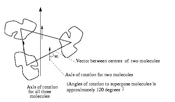
The diagram below shows what this means:
there are three molecules and the vectors between the centres of the molecules.
The direction of the axis of rotation to map one molecule onto another
is shown; it is at 90 degrees to the vector between the molecule centres.
To map one molecule onto the other needs some translation and a rotation
of approximately 120 degrees (in fact the angles are 131.3 degrees, 104
degrees and 131 degrees which are surprisingly different from 120 degrees).
This is right for a three-fold rotation axis and this shows there is a
rotation axis and not a screw axis. This helps to confirm that the solution
is correct because MolRep did not use this information to find the solution.

Alternative Stage 3) Run
aMoRe Molecular Replacement Program
Stage 4) Refine the Structure
It is not always certain that the molecular replacement is
correct - the best way to test it is to refine the model.
The best way to start refinement when there is more than one molecule in
the asymmetric unit is to use the non-crystallographic symmetry to restrain
the refinement - that is the refinement program must keep all the molecules
the similar.
and B
and C
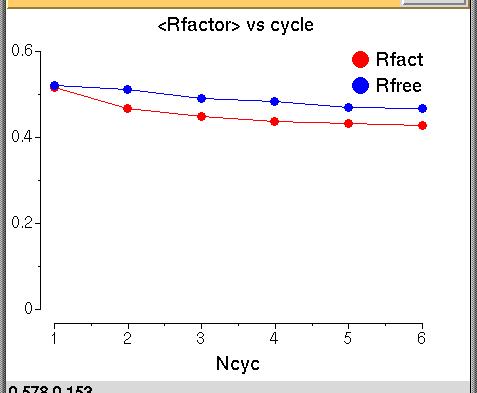
The graph shows the Rfactor (red) and the Free Rfactor
(blue) for 6 cycles of refinement. The Free Rfactor goes down from
52% to 46% The Rfactor is high - this is normal after
molecular replacement because we do not have a good model yet but
it goes down so we probably have a good solution.
To find out more:
MolRep: http://www.ysbl.york.ac.uk/~alexei/molrep.html
CCP4: http://www.dl.ac.uk/CCP/CCP4
Additional material: Peter Briggs & Martyn Winn, February 2001